Introduction
Load flow analysis, also known as power flow analysis, is a fundamental aspect of power system studies. It determines the steady-state voltages, real and reactive power flows, and power losses in a power network under normal operating conditions. This analysis is crucial for designing future expansions, optimizing existing networks, real-time monitoring, and contingency planning. Since the load flow problem is inherently non-linear, iterative numerical methods are required to solve it. Among the most commonly used techniques are the Gauss-Seidel Method and the Newton-Raphson Method.
Power Flow Problem Formulation
In a power system with multiple buses, each bus is categorized as:
- Slack Bus: Voltage magnitude and angle are specified (reference bus).
- PV Bus: Real power and voltage magnitude are specified.
- PQ Bus: Real and reactive powers are specified.
The power flow equations for bus ( i ) are:
[ P_i = \sum_{j=1}^{n} |V_i||V_j||Y_{ij}|\cos (\theta_{ij} + \delta_j – \delta_i) ]
[ Q_i = \sum_{j=1}^{n} |V_i||V_j||Y_{ij}|\sin (\theta_{ij} + \delta_j – \delta_i) ]
Where:
- ( V_i, V_j ) are voltages at buses ( i ) and ( j ).
- ( Y_{ij} ) is the element of the admittance matrix.
- ( \delta_i, \delta_j ) are voltage angles.
- ( \theta_{ij} ) is the angle of admittance.
These equations are non-linear and require iterative techniques for solutions.
Gauss-Seidel Method
The Gauss-Seidel method is an extension of the classical technique used for solving linear equations. It updates bus voltages sequentially and uses the latest values during the iteration.
Steps
- Initialize voltages for all buses (usually ( 1\angle0^\circ ) p.u.).
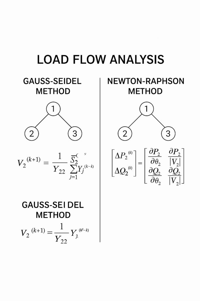
- Update each PQ bus voltage using:
[ V_i^{(k+1)} = \frac{1}{Y_{ii}} \left[ \frac{P_i – jQ_i}{(V_i^{(k)}){n} Y_{ij} V_j^{(k+1)} \right] ]
- Continue iterations until convergence is achieved (voltage change below tolerance).
Advantages
- Simple to understand and implement.
- Low memory requirement.
Disadvantages
- Slow convergence, especially for large systems.
- Sensitive to initial guess and ordering.
Newton-Raphson Method
The Newton-Raphson method uses a Taylor series expansion and Jacobian matrix to solve the power flow equations. It is more mathematically intensive but offers faster and more reliable convergence.
Steps
- Formulate a set of non-linear equations:
[ \mathbf{f}(x) = 0 ]
Where ( x = [\delta_2, …, \delta_n, V_{m+1}, …, V_n] ) is the state vector.
- Perform Taylor series expansion:
[ \mathbf{f}(x + \Delta x) \approx \mathbf{f}(x) + J(x) \Delta x = 0 \Rightarrow \Delta x = -J(x)^{-1} \mathbf{f}(x) ]
- Solve the linear system for ( \Delta x ) and update state variables.
- Iterate until ( \Delta x ) is less than the specified tolerance.
- Faster convergence.
- More reliable and accurate results.
- Requires fewer iterations.
- Complex programming.
- Higher memory requirements.
Conclusion
Load flow analysis is essential for power system planning and operation. The Gauss-Seidel method, though simple, is slow and less effective for large systems. The Newton-Raphson method, on the other hand, offers faster and more reliable convergence, making it the preferred choice for complex power networks. Selecting the appropriate method depends on system size, computational resources, and accuracy requirements.