Introduction
Electrical systems are fundamental to modern technology, spanning power generation, electronic circuits, communication networks, and control systems. Modeling these systems effectively allows engineers and researchers to analyze and predict behavior under various conditions. One of the most powerful methods for representing electrical systems is state-space modeling, which provides a framework for expressing system dynamics using state variables and matrix equations.
State-space modeling is particularly useful for time-domain analysis, multi-input multi-output (MIMO) systems, and digital control applications. Unlike classical transfer function models, state-space representation captures both the internal dynamics and external inputs affecting the system.
This article explores the fundamentals of state-space modeling, its application in electrical systems, conversion from circuit equations to state-space form, and the significance of state-space analysis in modern electrical engineering.
Overview of State-Space Representation
Definition
The state-space representation of a system is a mathematical model that expresses the system’s dynamics using a set of first-order differential equations. These equations describe how the system evolves over time based on its current state and external inputs.
The general form of a linear time-invariant (LTI) system in state-space notation is:
[ \dot{\mathbf{x}}(t) = \mathbf{A} \mathbf{x}(t) + \mathbf{B} \mathbf{u}(t) ]
[ \mathbf{y}(t) = \mathbf{C} \mathbf{x}(t) + \mathbf{D} \mathbf{u}(t) ]
where:
- (\mathbf{x}(t)) is the state vector, representing the system’s internal variables.
- (\dot{\mathbf{x}}(t)) is the derivative of the state vector, showing how states change over time.
- (\mathbf{u}(t)) is the input vector, representing external influences on the system.
- (\mathbf{y}(t)) is the output vector, representing observable system outputs.
- (\mathbf{A}) is the state matrix, defining internal system dynamics.
- (\mathbf{B}) is the input matrix, defining how inputs affect states.
- (\mathbf{C}) is the output matrix, defining how states affect outputs.
- (\mathbf{D}) is the feedthrough matrix, defining direct input-output relationships.
State-space modeling is advantageous because it provides a structured approach to controllability, observability, and stability analysis in electrical systems.
Application of State-Space Representation in Electrical Systems
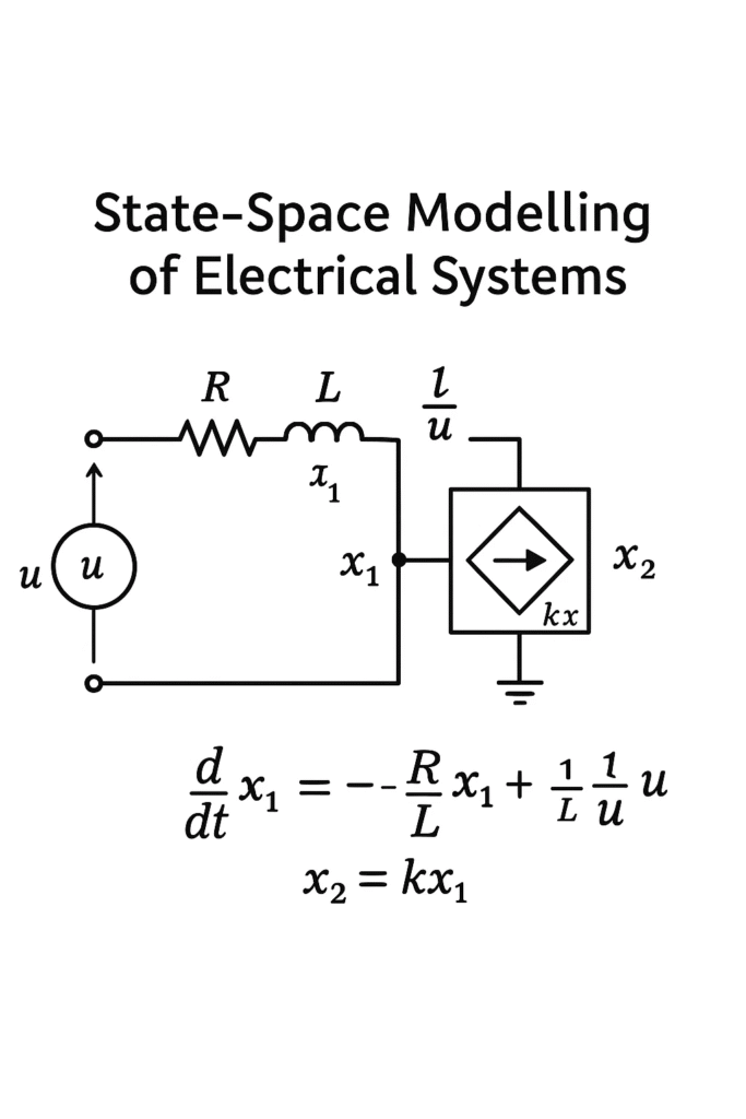
Electrical systems, including RLC circuits, DC motors, and power electronic converters, can be modeled using state-space equations. The key steps in developing a state-space model involve:
- Identifying state variables (e.g., voltages, currents).
- Deriving differential equations governing system behavior.
- Expressing equations in matrix form to obtain the state-space representation.
Example: State-Space Model of an RLC Circuit
Consider a series RLC circuit consisting of:
- Resistor ((R))
- Inductor ((L))
- Capacitor ((C))
with an input voltage (V_{in}(t)) and output voltage (V_{out}(t)) across the capacitor.
Using Kirchhoff’s Voltage Law (KVL):
[ V_{in}(t) = L \frac{dI}{dt} + R I + V_C ]
where:
- (I(t)) is the current.
- (V_C(t)) is the capacitor voltage, related by:
[ I = C \frac{dV_C}{dt} ]
Defining state variables:
[ x_1 = V_C, \quad x_2 = I ]
Rewriting in first-order differential form:
[ \frac{dx_1}{dt} = \frac{1}{C} x_2 ]
[ \frac{dx_2}{dt} = -\frac{R}{L} x_2 – \frac{1}{L} x_1 + \frac{1}{L} V_{in} ]
Thus, the state-space model is:
[ \dot{\mathbf{x}} = \begin{bmatrix} 0 & \frac{1}{C} \ -\frac{1}{L} & -\frac{R}{L} \end{bmatrix} \mathbf{x} + \begin{bmatrix} 0 \ \frac{1}{L} \end{bmatrix} V_{in} ]
[ \mathbf{y} = \begin{bmatrix} 1 & 0 \end{bmatrix} \mathbf{x} + \begin{bmatrix} 0 \end{bmatrix} V_{in} ]
This model allows engineers to simulate, analyze, and design controllers for electrical systems.
Advantages of State-Space Analysis in Electrical Engineering
- Systematic Approach to Modeling
- Handles multi-variable systems effectively.
- Supports time-domain analysis without requiring Laplace transforms.
- Controllability and Observability Analysis
- Determines whether a system can be fully controlled using input signals.
- Identifies if the system’s internal states are measurable from output signals.
- Stability and Performance Assessment
- Evaluates dynamic behavior using eigenvalues of the state matrix.
- Facilitates advanced control design, including optimal control and adaptive systems.
- Digital Control Applications
- Essential for modern embedded systems and microcontrollers.
- Enables discrete-time modeling for digital signal processing (DSP) and power electronics.
Challenges & Considerations in State-Space Modeling
Despite its advantages, state-space modeling requires careful formulation to ensure accuracy:
- Modeling Complexity
- High-order systems can lead to large matrix representations.
- Requires state reduction techniques for simplification.
- Parameter Identification
- Accurate estimation of system parameters ((R, L, C)) is critical.
- Experimental validation may be necessary.
- Numerical Computation Issues
- Requires matrix operations, which can be computationally expensive.
- Stability analysis depends on precise eigenvalue calculations.
Despite these challenges, state-space methods remain a cornerstone of modern electrical engineering, enabling efficient analysis, simulation, and control of electrical systems.

Conclusion
State-space modeling is a powerful mathematical tool for analyzing electrical systems. It provides a structured representation that captures both internal dynamics and external inputs, making it ideal for control system design and simulation.
By applying state-space methods, engineers can analyze RLC circuits, power electronics, and electromechanical systems, ensuring robust performance in real-world applications. Though challenges exist in parameter estimation and computational complexity, the benefits of state-space analysis far outweigh its limitations.
